딥러닝을 이용한 자연어처리 입문 #9-3. (08) 케라스의 SimpleRNN과 LSTM 이해하기 -(11) 문자 단위 RNN
(08) 케라스의 SimpleRNN과 LSTM 이해하기
1 SimpleRNN 이해하기
rnn - SimpleRNN (3)
# rnn = SimpleRNN (3, return_sequences-False, return_state=False)
hidden_state= rnn(train_X)
print('hidden state: {}, shape: {}'.format(hidden_state, hidden_state.shape))
# 출력값 : hidden state: [[-0.866719 0.95010996 -0.99262357]], shape: (1, 3)
마지막 시점의 은닉 상태
rnn = SimpleRNN(3, return_sequences=True)
hidden_states = rnn(train_X)
print('hidden states: {}, shape: {}'.format(hidden_states, hidden_states.
shape))
# 출력값 :hidden states: [[[ 0.92948684 -0.9985648 0.98355013]
#                         [ 0.89172053 -0.9984244 0.191779]
#                         [ 0.6681082 -0.96870355 0.6493537 ]
# [ 0.95280755 -0.98854564 0.7224146 ]]], shape: (1, 4, 3)- return_sequences = True로 지정하여 (1, 4, 3) 크기의 텐서 출력
SimpleRNN(3, return_sequences-True, return_state-True)
hidden_states, last_state= rnn(train_X)
print('hidden states: {}', shape: ().format(hidden_states, hidden_states.
shape))
print('last hidden state: {}, shape: {}'.format(last_state, last_state.sh
ape))
# hidden states: [[[ 0.29839835 -0.99608386 0.2994854 ]
#                [ 0.9160876 0.01154806 0.86181474]
#                [-0.20252597 -0.9270214 0.9696659]
#                [-0.5144398 -0.5037417 0.96605766]]], shape: (1, 4, 3)
#                last hidden state: [[-0.5144398 -0.5037417 0.96605766]], shape: (1, 3)
return_state = True로 인한 출력으로 마지막 시점의 은닉 상태
rnn - SimpleRNN (3, return_sequences-False, return_state-True)
hidden_state, last_state = rnn(train_X)
print('hidden state: {}, shape: {}'.format(hidden_state, hidden_state.sha
pe))
print('last hidden state: {}, shape: {}'.format(last_state, last_state.sh
ape))
# hidden state: [[0.07532981 0.97772664 0.97351676]], shape: (1, 3)
# last hidden state: [[0.07532981 0.97772664 0.97351676]], shape: (1, 3)
2 LSTM 이해하기
lstm= LSTM(3, return_sequences=False, return_state=True)
hidden_state, last_state, last_cell_state = 1stm(train_x)
print('hidden state: {}, shape: {}'.format(hidden_state, hidden_state.shape))
print('last hidden state: {}, shape: {}.format(last_state, last_state.shape))
print('last cell state: {}, shape: {}'.format (last_cell_state, last_cell_state.shape))
# hidden state [[-0.00263056 0.20051427 -0.22501363]], shape: (1, 3)
# last hidden state: [[-0.00263056 0.20051427 -0.22501363]], shape: (1, 3)
# last cell state: [[-0.04346419 0.44769213 -0.2644241 ]], shape: (1, 3)- SimpleRNN과는 달리 세개의 결과를 반환함
lstm = LSTM(3, return_sequences=True, return_state=True)
hidden_states, last_hidden_state, last_cell_state - 1stm(train_X)
print('hidden states: {}, shape: {}'.format(hidden_states, hidden_states.
shape))
print('last hidden state: {}, shape: {}'.format(last_hidden_state, last_h
idden_state.shape))
print('last cell state: {}, shape: {}'.format(last_cell_state, last_cell_
state.shape))
# hidden states [[[ 0.1383949 0.01107763 -0.00315794]
# [0.0859854 0.03685492 -0.01836833]
# [-0.02512104 0.12305924 -0.0891041 ]
# [-0.27381724 0.05733536 -0.04240693]]], shape: (1, 4, 3)
# last hidden state: [[-0.27381724 0.05733536 -0.04240693]], shape: (1, 3)
# last cell state: [[-0.39230722 1.5474017 -0.6344505 ]], shape: (1, 3)- return_sequences = True로 설정하여 셀 상태까지 반환함
3 Bidirectional(LSTM) 이해하기
k_init = tf.keras.initializers.Constant(value=0.1)
b_init = tf.keras.initializers.Constant (value=0)
r_init = tf.keras.initializers.Constant(value=0.1)
return_sequences> False 01, return_state True 44.
bilstm - Bidirectional (LSTM(3, return_sequences-False, return_state-True,init, recurrent_initializer=r_init))
hidden_states, forward_h, forward_c, backward_h, backward_c = bilstm(trail_X)
kernel_initializer-k_init, bias_initializer-b
print('hidden states: {}, shape: {}'.format(hidden_states, hidden_statesshape))
print('forward state: {}, shape: {}'.format(forward_h, forward_h.shape))
print("backward state: {}, shape: {}.format(backward_h, backward_h.shape))
# hidden states: [[0.6303139 0.6303139 0.6303139 0.70387346 0.703873460.70387346]], shape: (1, 6)
# forward state: [[0.6303139 0.6303139 0.6303139]], shape: (1, 3)
# backward state: [[0.70387346 0.70387346 0.70387346]], shape: (1, 3)
(9) RNN 언어 모델
RNN 언어 모델
RNN은 언어 모델을 만들면 입력의 길이를 고정하지 않을 수 있음
[테스트 과정]

[훈련 과정(교사 강요)]
what will the fat cat sit on라는 훈련 샘플이 있다면,
what will the fat cat sit 시퀀스를 모델의 입력으로 넣으면, will the fat cat sit on를 예측하도록 훈련됨
- 훈련 과정 동안 출력층에서 사용하는 활성화 함수는 소프트맥스 함수
- 모델이 예측한 값과 실제 레이블과의 오차를 계산하기 위한 손실 함수로 크로스 엔트로피 함수를 사용함
[RNNLM 시각화]
(10) RNN을 이용한 텍스트 생성
RNN을 이용하여 텍스트 생성하기
- ‘경마장에 있는 말이 뛰고 있다’
- ‘그의 말이 법이다’
- ‘가는 말이 고와야 오는 말이 곱다’
import numpy as np
from tensorflow.keras.preprocessing.text import Tokenizer
from tensorflow.keras.preprocessing.sequence import pad_sequences
from tensorflow.keras.utils import to_categorical
text = """경마장에 있는 말이 뛰고 있다\n 그의 말이 법이다\n 가는 말이 고와야 오는 말이 곱다\n"""
tokenizer Tokenizer()
tokenizer.fit_on_texts([text])
vocab_size = len(tokenizer.word_index) + 1
print('93%d % vocab_size)
# 단어 집합의 크기 : 12- 각 단어와 단어에 부여된 정수 인덱스 출력
print(tokenizer.word_index)
# {'말미': 1, '경마장에': 2, '있는': 3, '뛰고': 4, '있다': 5, '그의': 6, '법이다' : 7, '가는': 8, '고와야': 9, '오는': 10, '곱다' : 11}- 훈련 데이터 만들기
sequences = list()
for line in text.split('\n'):
	encoded tokenizer.texts_to_sequences([line])[0]
	for i in range(1, len(encoded)):
		sequence encoded[:1+1]
		sequences.append(sequence)

print('학습에 사용할 샘플의 개수 %d' % len(sequences))

# 학습에 사용할 샘플의 개수: 11
print (sequences)
# [[2, 3], [2, 3, 1], [2, 3, 1, 4], [2, 3, 1, 4, 5], [6, 1], [6, 1, 7], [8,
# 1], [8, 1, 9], [8, 1, 9, 10], [8, 1, 9, 10, 1], [8, 1, 9, 10, 1, 11]]- 전체 샘플에 대해서 길이를 일치시켜 줌
max_len - max(len(1) for 1 in sequences) # 모든 샘플에서 길이가 가장 긴 샘플의 길이 출력
print('샘플의 최대 길이 : {}'.format(max_len))
# 샘플의 최대 길이 : 6- 길이를 6으로 패딩
sequences pad_sequences (sequences, maxlen-max_len, padding="pre")
print (sequences)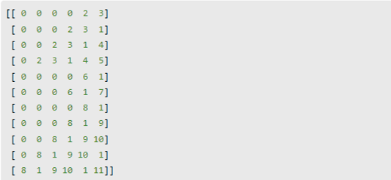
- X와 y분리
sequences np.array(sequences)
X = sequences[:,:-1]|
y = sequences[:,-1]

분리된 X와 y에 대해서 출력해보면 다음과 같습니다.
- 레이블에 대해 원핫인코딩
y = to_categorical(y, num_classes-vocab_size)
원-핫 인코딩이 수행되었는지 출력합니다.
print(y)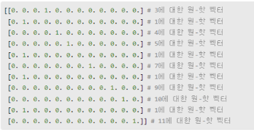
2) 모델 설계하기
하이퍼 파라미터인 임베딩 벡터의 차원은 10, 은닉 상태의 크기는 32
embedding_dim 10
hidden_units = 32
model Sequential()
model.add(Embedding (vocab_size, embedding_dim))
model.add(SimpleRNN(hidden_units))
model.add(Dense(vocab_size, activation='softmax'))
model.compile(loss='categorical_crossentropy', optimizer-'adam', metrics-['accuracy'])
model.fit(x, y, epochs-200, verbose=2)
모델이 정확하게 예측하고 있는지 문장을 생성하는 함수를 만들어서 출력
def sentence_generation(model, tokenizer, current_word, n): #모델, 토크나이저, 현재 단어, 반복할 횟수
	init_word current_word
	sentence =''

	#n번 반복
	for in range(n):
		# 현재 단어에 대한 정수 인코딩과 패딩
		encoded - tokenizer.texts_to_sequences([current_word])[e]
		encoded = pad_sequences([encoded], maxlen=5, padding="pre")
		# 입력한 X(현재 단어)에 대해서 Y를 예측하고 Y예측한 단어) result에 저장.
		result = model.predict(encoded, verbose=0)
		result = np.argmax(result, axis-1)

			for word, index in tokenizer.word_index.items():
			# 만약 예측한 단어와 인덱스와 동일한 단어가 있다면 break
			if index = result:
				break

            # 현재 단어 + + 예측 단어를 현재 단어로 변경
			current_word current_word +'' + word

			# 예측 단어를 문장에 저장
			sentence = sentence + '' + word

    sentence = init_word + sentence
	return sentence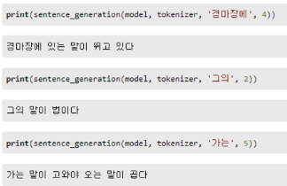
(11) 문자 단위 RNN
문자 단위 RNN 언어 모델(Char RNNLM)
1) 데이터에 대한 이해와 전처리
import numpy as np
import urllib.request
from tensorflow.keras.utils import to categorical

# 데이터 로드
urllib.request.urlretrieve("http://www.gutenberg.org/files/11/11-0.txt", filename-"11-0.txt")

f= open('11-0.txt', 'rb')
sentences = []
for sentence in : 데이터로부터 한 줄씩 읽는다.
	sentence=sentence.strip() # strip()
	sentence=sentence.lower() # 48X2.
	sentence=sentence.decode('ascii', 'ignore') # \xe2\x80\x99 바이트 열 제거

    if len(sentence) > 0:
		sentences.append(sentence)
f.close()
total_data= ''.join(sentences)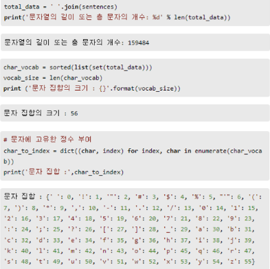
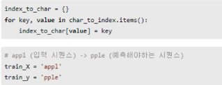
정수로부터 문자를 리턴하는 index_to_char 만들기
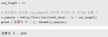
15만 9천의 길이를 가진 문자열로부터 다수의 샘플 만들기
'공부하는 습관을 들이자 > Deep Learning (NLP,LLM)' 카테고리의 다른 글
| [딥러닝 자연어처리] 11. 8) 사전 훈련된 워드 임베딩 ~ 09) 사전 훈련된 워드 임베딩 사용하기 (0) | 2024.01.02 |
|---|---|
| [딥러닝 자연어처리] 10. (1) 워드 임베딩 ~ 7) 자모 단위 한국어 fast text 학습하기 (0) | 2024.01.01 |
| [딥러닝 자연어처리] 9-2. (05) 양방향 순환 신경망 - (07) 게이트 순환 유닛 (0) | 2023.12.26 |
| [딥러닝 자연어처리] 9-1. (01) 순환 신경망 (Recurrent Neural Network) (0) | 2023.12.25 |
| [딥러닝 자연어처리] 8-6. (08) 케라스의 함수형 API - (10)다층 퍼셉트론으로 텍스트 분류하기 (0) | 2023.12.22 |


